Abstract
We propose an efficient and unified framework, namely ThiNet, to simultaneously accelerate and compress CNN models in both training and inference stages. We focus on the filter level pruning, i.e., the whole filter would be discarded if it is less important. Our method does not change the original network structure, thus it can be perfectly supported by any off-the-shelf deep learning libraries. We formally establish filter pruning as an optimization problem, and reveal that we need to prune filters based on statistics information computed from its next layer, not the current layer, which differentiates ThiNet from existing methods. Experimental results demonstrate the effectiveness of this strategy, which has advanced the state-of-the-art. We also show the performance of ThiNet on ILSVRC-12 benchmark. ThiNet achieves 3.31x FLOPs reduction and 16.63x compression on VGG-16, with only 0.52% top-5 accuracy drop. Similar experiments with ResNet-50 reveal that even for a compact network, ThiNet can also reduce more than half of the parameters and FLOPs, at the cost of roughly 1% top-5 accuracy drop. Moreover, the original VGG-16 model can be further pruned into a very small model with only 5.05MB model size, preserving AlexNet level accuracy but showing much stronger generalization ability.
1. Overview
1.1 Framework of ThiNet
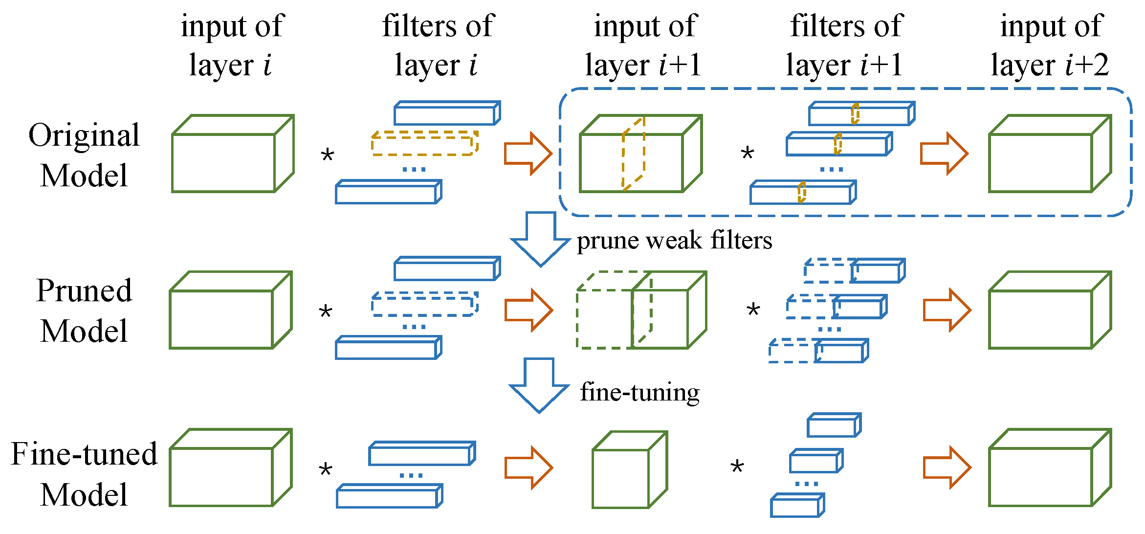
Figure 1. Illustration of ThiNet. First, we focus on the dotted box part to determine several weak channels and their corresponding filters (highlighted in yellow in the first row). These channels (and their associated filters) have little contribution to the overall performance, thus can be discarded, leading to a pruned model. Finally, the network is fine-tuned to recover its accuracy.
1.2 Collecting training examples
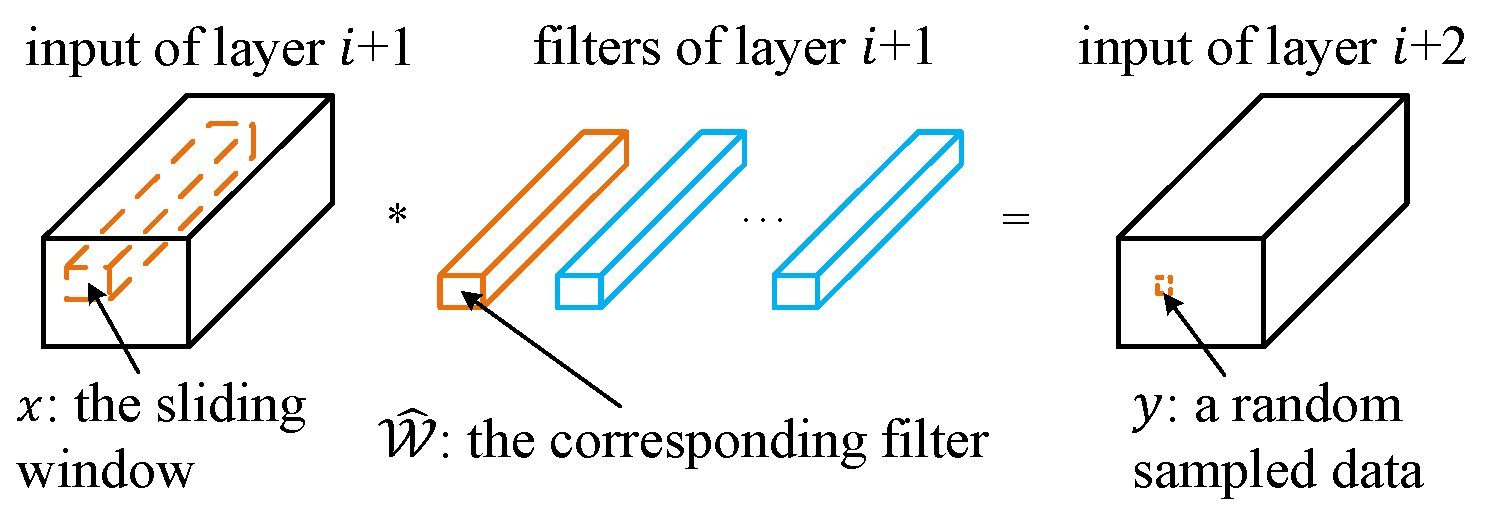
Normally, the convolution operation can be computed with a corresponding bias $b$ as follows:
\begin{equation}
    y = \sum_{c=1}^C\sum_{k_1=1}^K\sum_{k_2=1}^K\widehat{\mathcal{W}}_{c,k_1,k_2}\times x_{c,k_1,k_2}+b.
    \end{equation}
Now, if we further define:
\begin{equation*}
    \hat{x}_c=\sum_{k_1=1}^K\sum_{k_2=1}^K\widehat{\mathcal{W}}_{c,k_1,k_2}\times x_{c,k_1,k_2}
    \end{equation*}
Eq.1 can be simplified as: \(\hat{y} = \sum_{c=1}^C\hat{x}_c\), where \(\hat{y} = y - b.\) If we can find a subset \(S \subset \{1,2,\ldots, C\}\), and the equality
\begin{equation}
    \hat{y} = \sum_{c \in S}\hat{x}_c
    \end{equation}
always holds, then we do not need any \(\hat{x}_c\) if \(c \notin S\). Hence, these channels can be safely removed without changing the CNN model's result.
Of course, Eq. 2 cannot always be true for all instances of the random variables \(\hat{x}\) and \(\hat{y}\). However, we can manually extract instances of them to find a subset \(S\) such that Eq. 2 is approximately correct.
1.3 A greedy algorithm for channel selection
Now, given a set of \(m\) (the product of number of images and number of locations) training examples \(\{(\mathbf{\hat{x}}_i, \hat{y}_i)\}\), the original channel selection problem becomes the following optimization problem:
\begin{equation}
      \begin{aligned}
      \mathop{\arg\min}\limits_{S}  & \sum_{i=1}^{m}\left(\hat{y}_i-\sum_{j\in S}\mathbf{\hat{x}}_{i,j}\right)^2\\
      \text{s.t.}\quad & |S|=C\times r, \quad S \subset \{1,2,\ldots, C\}.
      \end{aligned}
      \end{equation}
Here, \(|S|\) is the number of elements in a subset \(S\), and \(r\) is a pre-defined compression rate (i.e., how many channels are preserved). Equivalently, let \(T\) be the subset of removed channels (i.e., \(S\cup T=\{1,2,\ldots,C\}\) and \(S\cap T=\emptyset\)), we can minimize the following alternative objective:
\begin{equation}
      \begin{aligned}
      \mathop{\arg\min}\limits_{T} & \sum_{i=1}^{m}\left(\sum_{j\in T}\mathbf{\hat{x}}_{i,j}\right)^2\\
      \text{s.t.}\quad & |T|=C\times (1-r), \quad T \subset \{1,2,\ldots, C\}.
      \end{aligned}
      \end{equation}
Eq. 4 is equivalent to Eq. 3, but has faster speed because $|T|$ is usually smaller than $|S|$. Solving Eq. 3 is still NP hard, thus we propose a greedy strategy (algorithm 1).
1.4 Minimize the reconstruction error
we can further minimize the reconstruction error (c.f. Eq. 3) by weighing the channels, which can be defined as:
\begin{equation}
      \mathbf{\hat{w}}=\mathop{\arg\min}\limits_{\mathbf{w}}\sum_{i=1}^{m}(\hat{y}_i- \mathbf{w}^\mathrm{T}\mathbf{\hat{x}}^*_i)^2.
      \end{equation}
Eq. 5 can be solved using the ordinary least squares approach: $\mathbf{\hat{w}} = (\mathbf{X}^\mathrm{T}\mathbf{X})^{-1}\mathbf{X}^\mathrm{T}\mathbf{y}$.
2. Experimental Results
2.1 Different filter selection criteria

Figure 3. Performance comparison of different channel selection methods: the VGG-16-GAP model pruned on CUB-200 with different compression rates.
2.2 VGG16 on ImageNet
Table 1. Results of VGG-16 on ImageNet using ThiNet. Here, M/B means million/billion ($10^6$/$10^9$), respectively; f./b. denotes the forward/backward timing in milliseconds tested on one M40 GPU with batch size 32.
| Model | Top-1 | Top-5 | #Param. | #FLOPs | f./b. (ms) |
|---|---|---|---|---|---|
| Original1 | 68.34% | 88.44% | 138.34M | 30.94B | 189.92/407.56 |
| ThiNet-Conv | 69.80% | 89.53% | 131.44M | 9.58B | 76.71/152.05 |
| Train from scratch | 67.00% | 87.45% | 131.44M | 9.58B | 76.71/152.05 |
| ThiNet-GAP | 67.34% | 87.92% | 8.32M | 9.34B | 71.73/145.51 |
| ThiNet-Tiny2 | 59.34% | 81.97% | 1.32M | 2.01B | 29.51/55.83 |
| SqueezeNet [15] | 57.67% | 80.39% | 1.24M | 1.72B | 37.30/68.62 |
1For a fair comparison, the accuracy of original VGG-16 model is evaluated on single center-cropped images (first resize to 256$\times$256) using pre-trained model as adopted in [10, 14]. Hence its accuracy would be slightly lower than some reports.
2Note that there are two different strategies to organize ImageNet dataset:
For a fair comparison, we follow previous work to organize dataset with "fixed size" strategy in most model. However, the "keep aspect ratio" strategy is more popular in real application, we train ThiNet-Tiny model on this dataset.
- fixed size: each image is firstly resized to 256$\times$256, then center-cropped to obtain a 224$\times$224 regin;
- keep aspect ratio: each image is firstly resized with shorter side=256, then center-cropped;
Table 2. Comparison among several state-of-the-art pruning methods on the VGG-16 network. Some exact values are not reported in the original paper and cannot be computed, thus we use $\approx$ to denote the approximation value.
| Model | Top-1 | Top-5 | #Param. $\downarrow$ | #FLOPs $\downarrow$ |
|---|---|---|---|---|
| APoZ-1 [14] | -2.16% | -0.84% | 2.04$\times$ | $\approx$1$\times$ |
| APoZ-2 [14] | +1.81% | +1.25% | 2.70$\times$ | $\approx$1$\times$ |
| Taylor-1 [23] | - | -1.44% | $\approx$1$\times$ | 2.68$\times$ |
| Taylor-2 [23] | - | -3.94% | $\approx$1$\times$ | 3.86$\times$ |
| ThiNet-WS [21] | +1.01% | +0.69% | 1.05$\times$ | 3.23$\times$ |
| ThiNet-Conv | +1.46% | +1.09% | 1.05$\times$ | 3.23$\times$ |
| ThiNet-GAP | -1.00% | -0.52% | 16.63$\times$ | 3.31$\times$ |
3. Additional results
3.1 Computational complexity of pruning process
Our pruning process is constituted by two major parts: feature extraction and channel selection.
As for the size of matrix (used for channel selection in section 3.2.2), it takes up 51.2MB disk space when channel number is 64 and 409.6MB with 512 channels. These costs are negligible compared to fine-tuning or training the network from scratch.
- The former depends on model inference speed, which takes 769.37s on one M40 GPU using the original VGG-16 model.
- The latter is determined by the number of filters in the current layer (64 in conv1_1, 512 in conv4_3). We test the computational cost of these two layers, which takes 2.34s and 137.36s respectively.
3.2 The effect of fine-tuning
We removed 60% filters in conv1_1 of VGG-16-GAP model (similar experimental setting as section 4.1) with different selection methods, and fine-tuned the pruned model in one epoch. The accuracy changes (tested on CUB-200) before/after fine-tuning are listed as follows:| Method | Before fine-tuning | After fine-tuning |
|---|---|---|
| random | 51.26% | 67.83% |
| weight sum [21] | 40.99% | 63.72% |
| APoZ [14] | 58.16% | 68.78% |
| ThiNet w/o w | 68.24% | 70.38% |
| ThiNet | 70.75% | 71.11% |
Hence, fine-tuning is important to recover the model accuracy in these methods, and ThiNet seems relatively robust than others.
4. Supplemental materials
We provide additional results and discussion in the supplemental document.
References
Jian-Hao Luo, Jianxin Wu, and Weiyao Lin: ThiNet: A Filter Level Pruning Method for Deep Neural Network Compression
To appear in International Conference on Computer Vision (ICCV), 2017.
@inproceedings{iccv2017ThiNet,
title={{ThiNet: A Filter Level Pruning Method for Deep Neural Network Compression}},
author={Jian-Hao Luo, Jianxin Wu, and Weiyao Lin},
booktitle={International Conference on Computer Vision (ICCV)},
month={October},
year={2017}
}